7. Magnetic Fields #
So far we have covered the important mathematical properties of static electric fields - that is the electric fields arising from stationary charges. No we are going to look at static magnetic fields. From an early age, even before you studied physics, you were probably acquainted with magnets, in toys for example. But what exactly is a magnetic field and where does it come from?
It is tempting to think of the magnetostatic field in the same way as an electrostatic field. You will often see it described in terms of ‘north’ and ‘south’ poles, principly by reference to the Earth’s magnetic field. However, this suggests the existence of what we might think of as magnetic charges. However, experience tells us that if we try to isolate these ‘charges’ by cutting a simple bar magnet in half say, we find we are never able to isolate, for example, a north pole.
A better starting point is to consider experiments that were found to produce magnetic fields by passing electrical currents through wires, and, in analogy to Coulomb’s law, characterising the magnetic field in terms of the force on one current carrying wire by another current carrying wire. In doing this we need to think carefully about what we mean by a current in a wire. In our normal description of current in a metal we think of the free movement of charges (electrons) through the metal while \(\textit{keeping the overall charge on the wire zero}\).
An alternative description might be in terms of a continuous (dense) charge carrying (i.e. electrons) beam in a vacuum. We refrain from talking about currents in this way for the moment for the following reason: although we can describe a current as the movement of charges in this beam, we note that any section of the beam would have an overall charge density as well and hence we would need to ask about the nature of the electric field from the beam as well. We could think a little more deeply and imagine that we are in a moving frame of reference in which these charges would appear stationary - i.e. what has happened to the magnetic field in this frame of reference! We can only really answer this questions when we start to apply the theory of special relativity (that you have just seen), but it turns out there is no contradiction apart from recognising electric and magnetic fields should really be considered together in terms of the electromagnetic field - something we will see later.
So at the start we will give our classical description of magnetostatic fields as arising from charges moving in overall electrically neutral wires.
7.1 Magnetic field lines
The simplest magnetic field that we might produce is from the ‘infinite’ straight wire carrying a current \(I\). What does the magnetic field look like? Well, the conclusion from work in the 19th century is that the field looks like this. We’ll not go into details about how they did this!
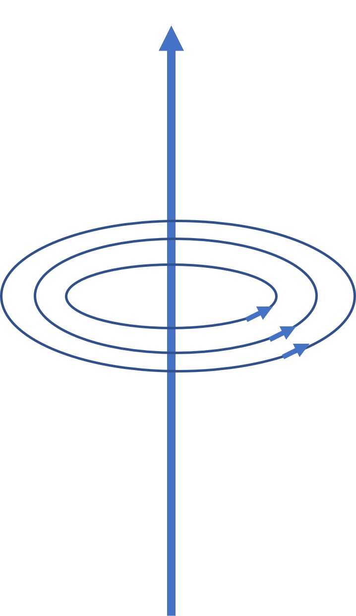
The first thing we note is that the field lines form continuous loops. They don’t seem to begin and end on any sources or sinks of a field. This is an important observation that we will return to. The second is the direction of the field lines follows a ‘right hand screw’ rule. (This is a convention from our definition of the direction of current).
7.2 Lorentz Force
If we place two current carrying wires parallel to each other we find that they exert a mutual force between them. We understand the origin of this force from the result of measurements of the motion of charged particles in magnetic fields for which the conclusion is,
\(\displaystyle\vec{F}=Q(\vec{v}\times\vec{B})\)
You may well have seen this result before as \(F=Bqv\) from which you used Flemming’s rules to work out the direction of the force. You may even have come across \(F=Bqv\sin(\theta)\) for the case that \(B\) was not perpendicular \(v\) - you would have described the direction. When we use the cross product to describe the force we no longer need to remember whether we use the left or right hand rule, the direction is given by the axial vector of the cross product. The only thing we have to remember is the order \(\vec{v}\) then \(\vec{B}\) in the formula. After a time writing \(\vec{F}=Q(\vec{B}\times\vec{v})\) just doesn’t look right (c.f. \(\vec{L}=\vec{r}\times\vec{p}\) not \(\vec{L}=\vec{p}\times\vec{r}\)). Note, this force law was determined (like Coulomb’s law) from careful observation - it is not derived from any higher principle.
Hence in the presence of Electrostatic and Magnetostatic fields we can write the force on a small test charge as,
###.
This is known as the \(\textit{Lorentz Force Law}\) and together with Maxwell’s equations (that we are working towards) is all that we need for the description of classical electromagnetism.
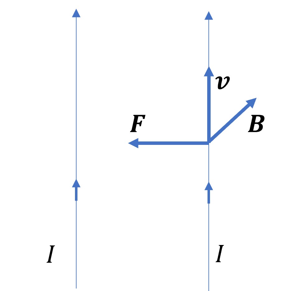
The figure shows how the magnetic part of the Lorentz force produces a force between two current carrying wires. The left hand current carrying wire produces a magnetic field at the second wire. The current in the second wire consists of charges moving with velocity \(\vec{v}\) along it. According to the Lorentz force this produces an attractive force between them. Reversing the current in either wire causes the direction of the force, the result of the cross product, to change direction and we get repulsion between the two wires.
7.3 Work done by magnetic fields
We saw in the case of the electric field that work had to be done on or by the charge to move it through the field. What happens as we move the charge through a magnetic field (we already know it will be deflected, not accelerated along its direction of motion). Well, work done (if no electric field is present) is given by,
\(\displaystyle dW = \vec{F}.d\vec{l}=Q(\vec{v}\times\vec{B})\cdot \vec{v}\,dt = 0\)
Make sure you understand this result by thinking about the direction of \(\vec{v}\times\vec{B}\) and \(\vec{v}\) and what the result of the dot product between them will be.
Hence, we find that \(\textit{Magnetic fields do no work}\). It is easy to forget this sometimes, but careful analysis in real cases reveals the true source of any work done as charges ae moved around. Griffiths gives some nice examples.
7.4 Current
As we saw above, our understanding of the origin of magnetic fields is due to the flow of currents. At the moment we can think of this in the conventional way in which the current is \(\textit{carried}\) by a wire. Our wire is a metal in which currents can flow freely (we will consider the role of resistance later). The current is then defined as the amount of charge passing per unit time through a point in the wire and has the units of Coulombs\(\cdot\)s\(^{-1}\) or the Ampere (A). Note, in this scenario there is no overall charge on the wire, so although charges are moving there is no \(\vec{E}\) field around the wire*. We now understand the current as due to electrons flowing in the wire.
To start with, our wire is conceptually considered as infinitely thin (c.f. a point charge in electrostatics) with no physical size of its own.
We can think of our current as a uniform line charge density moving through the wire with some speed \(v\) so that our current is
\(\displaystyle I=\lambda v\).
Now our wire does not have to be straight, it can have bends, loops etc. in it so we should realise that we need to not only specify the magnitude of the current (as above) but also its direction. This is easily achieved by changing the speed to velocity and hence,
\(\displaystyle \vec{I}=\lambda \vec{v}\).
We can combine this result with the Lorentz force (in the absence of \(\vec{E}\)) to find the magnetic force on a current carrying wire as,
\(\displaystyle \vec{F}_{magnetic}=\int (\vec{v}\times\vec{B})dq=\int(\vec{v}\times\vec{B})\lambda\; dl = \int (\vec{I}\times\vec{B}) dl\)
More commonly this is written as
###where we consider \(I\) as a scalar quantity but with the vectorial property of the current represented in the vector element \(d\vec{l}\) along the wire.
N.B. Note the order of the vectors in the cross-product. If you keep to this convention you will not get the direction of the force incorrect.
Exercise. At your school (at least for A level students) you will have come across the expression \(F=BIL\sin \theta\) for the force on a current carrying wire in a magnetic field. Derive this result from equation (7.2).
* As noted earlier, we will avoid for the moment, discussion of currents from,for example, beams of charged particles for which we need to worry about the electrostatic field as well.
7.5 Surface and volume current density.
In our consideration of electrostatics we found it more useful to talk about charge in terms of continuous charge, surface or line densities rather than in terms of individual charges. For the case of electric currents and our study of magnetic fields we find it useful to extend our idea of a current in an (infinitesimally small) wire to one of current flowing over a surface of finite size (sirface currents) or the current flowing through a surface in a solid section. i.e.
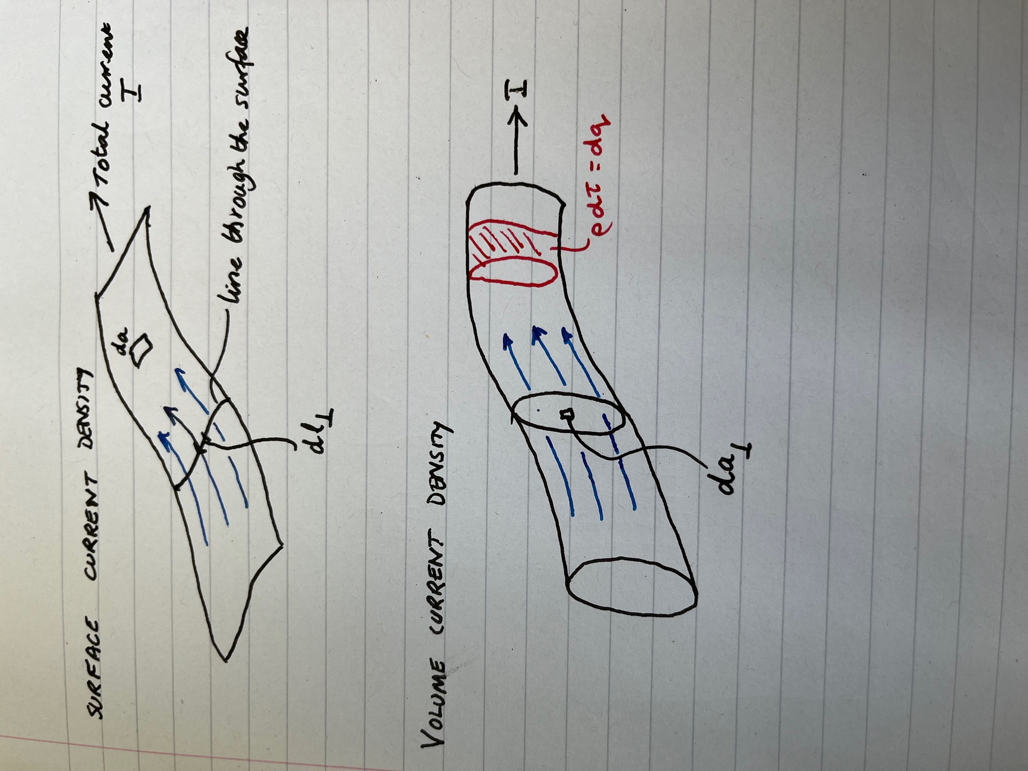
7.5.1 Surface current density
The figure shows our depiction of a current (depicted by the blue lines) flowing over a surface. We can see that the total current \(I\) flowing over the surface may be depicted in terms of the current flowing through a line on the surface. The current \(dI\) passing through any small element of this line \(dl_\perp\) is then d\(\vec{I}=\vec{K}dl_\perp\) where the vector direction of the current is perpendicular to the line. If we consider the velocity of the charges going through this line we can write this alternatively as
###,
where \(\vec{K}\) is the surface current density.
From this we can work out the total force on the surface in an external field \(\vec{B}\) as,
\(\displaystyle \vec{F}_{magnetic}=\int(\vec{v}\times\vec{B})\sigma da = \int (\vec{K}\times\vec{B})da\)
7.5.2 Volume current density
In a similar way we can define a volume current density. In this case we consider a total current \(I\) flowing through a cross-section of a wire for example. This cross section defines a surface. The current \(dI\) passing through an infinitesimal area, \(da_\perp\), on the this surface, where the vector direction of the current is perpendicular to the surface is \(\displaystyle d \vec{I} = J\;da_\perp\), so we write,
###,
where \(\vec{J}\) is the volume current density.
In this case we can write the force on the wire as,
\(\displaystyle \vec{F}_{magnetic} = \int(\vec{v}\times\vec{B})\rho d\tau = \int(\vec{J}\times\vec{B})d\tau\)
7.6 The continuity equation
From our definition of the current density \(\vec{J}\) we can write that the the current through a surface \(S\) is,
\(\displaystyle I = \int_S J\;da_\perp = \int_S \vec{J}.d\vec{a}\)
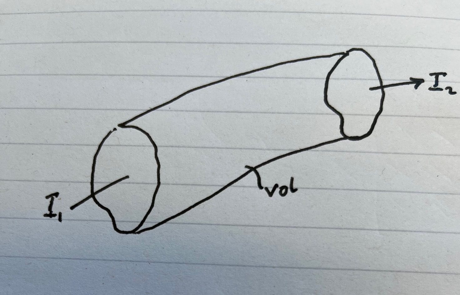
Now consider an enclosed volume, as shown in the figure. If current, doesn’t flow out of the ‘sides’ then we can consider the integration of \(\vec{J}\) over the enclosing surface shown. Hence,
\(\displaystyle \oint \vec{J}.d\vec{a} =\int_{Vol} \nabla\cdot\vec{J}d\tau\),
the right-hand side of the equation comong from the divergence theorem wher \(Vol\) is the volume enclosed. Given no current flows out of the sides (this does not have to be true but makes the argument easier to follow) the left handside corresponds to the net current (\(I_2-I_1\)) leaving the enclose volume, or in terms of the charge, the net charge leaving the volume per unit time. Hence we can write,
\(\displaystyle \int_{Vol}(\nabla \cdot \vec{J})d\tau = -\frac{d}{dt}\int_{Vol}\rho d\tau=-\int_{Vol}\left(\frac{\partial \rho}{\partial t}\right) d \tau\).
The minus comes about as the charge density decreases as charge flows out. From this we obtain the continuity equation,
###In words, if we consider a volume where currents are flowing then, if there is a net current into the volume, there must be a charge build up within that volume over time, and vice versa.
In this section we are considering magnetostatics - a regime where the magnetic fields do not vary with time. Hence the currents flowing must be steady. In other words \(\partial \rho / \partial t = 0\) and \(\partial \vec{J}/\partial t =0\). From this and the continuity equation we must have
\(\displaystyle \nabla \cdot \vec{J} = 0\)
for steady currents.