8. Properties of Magnetic Fields
In the previous section we explained that magnetic fields originate from electric currents and we described the forces acting on charged particles in these fields. We then took a little time to see how we could define the currents more precisely in terms of surface or volume current densities and introduced the continuity equation. Finally we stated the condition \(\nabla \cdot \vec{J}=0\) for steady currents required when considering magnetostatics. In this section we will explore further the properties of the magnetic field, in a similar way to our consideration of electrostatic fields, to show that likewise we can define \(\vec{B}\) in terms of simple expressions involving divergence and curl.
8.1 The Biot-Savart Law
In this section we must remember that we are considering the case of \(\textit magnetostatics\) that means we have in particular, \(\frac{\partial \rho}{\partial t}=0\) and \(\frac{\partial \vec{J}}{\partial t}=0\). We don’t really ask how we arrived at these condition. Note, in this consideration moving point charges are not considered as a current. With these constraints, the continuity equation gives \(\nabla \cdot \vec{J}=0\).
The relationship between the source of the magnetic field and the currents was first discovered experimentally and described by what is known as the \(\textit Biot-Savart\) law,
###It plays a similar role to Coulomb’s law in electrostatics. We can also express it in terms of a scalar current and the vector element along our current carrying wire.
###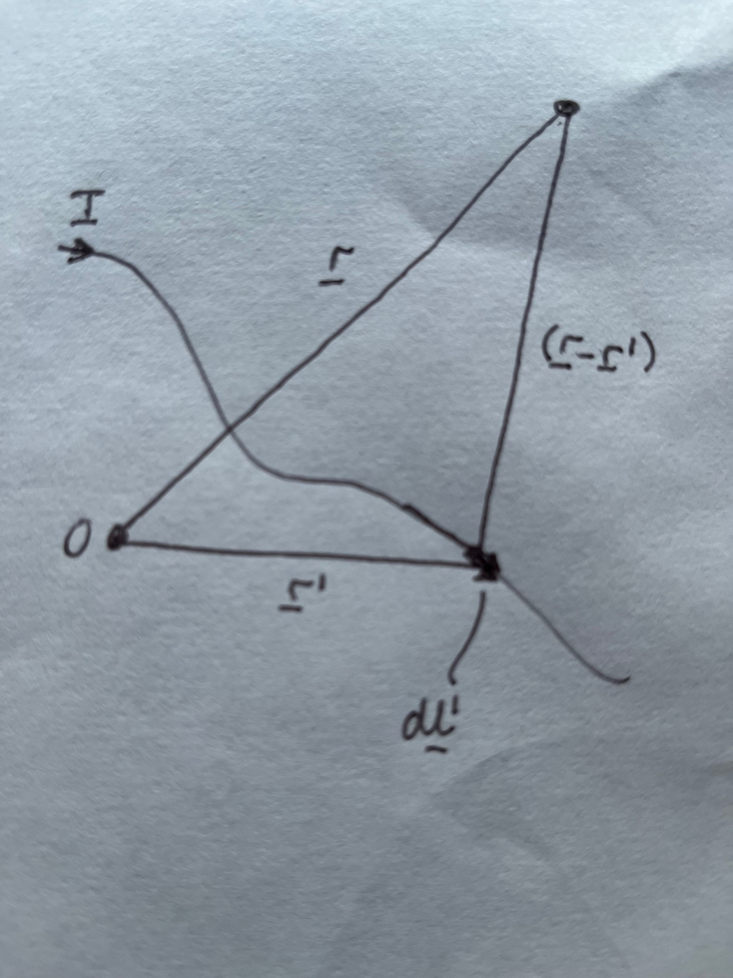
This integral has the same form as we have seen for the electric field from the charge distribution when we were considering electrostatics. The figure shows its interpretation. We are considering a point at position vector \(\vec{r}\) from the origin. The kernel of the integral represents the field that is produced from a small vector element of current \(I d\vec{l}\) at the poistion \(\vec{r'}\) remembering that the position vector of the point P from the element is \(\vec{r}-\vec{r'}\). Note, in 3D there are three parts to this integral for each spatical direction. In general this integral will be quite difficult to solve analytically (you will see a few examples) but it can always be solved numerically. As in the case of the electrostatic equivalents, careful choice of the origin simplifies the solutions. Take a little time to understand the structure of this integral and then see how it is applied in the example cases.
Note we have introduced a new physical constant, the permeability of free space, that is defined as,
\(\displaystyle \mu_0 = 4 \pi \times 10^{-7} N\cdot A^{-2}\).
The magnetic field is measured in units of Tesla (\(T\)) where,
\(\displaystyle 1T = 1 N\cdot A^{-1} \cdot m^{-1}\).
Note, the Biot-Savart law implies the superposition principle for magnetic fields - the addition of any new current elements just adds linearly to the field.
Exercise. Use the Biot-Savart law to show that the magnitude of the magnetic field at a distance \(s\) from an infinite long straight wire is,
\(\displaystyle B=\frac{\mu_0 I}{2 \pi s}\).
Use the Biot-Savart or the right hand rule to find the direction of the field and sketch the field lines.
8.2 Ampere’s law.
If we take our result for the magnetic field from a long straight wire that we gave in section 8.1 then we find,
\(\displaystyle \oint \vec{B}.d\vec{l}=\oint \frac{\mu_0 I}{2 \pi s}dl=\frac{\mu_0 I}{2 \pi s}\oint dl= \mu_0 I\),
where we have take a circular path of radius \(s\) around the wire. This result may be generalised (the proof is in Griffith’s section 5.3.2) to show that any path that encloses a total current \(I_{enclosed}\) gives rise to the result,
###that is known as \(Amp\grave{e}re's\) law. Note. the result of the integral is \(0\) if no current is enclosed.
8.3 The curl of \(\vec{B}\)
We may express the current in the wire of Amp\(\grave{e}\)re’s law in terms of the current density as,
\(\displaystyle I_{enclosed} = \int \vec{J} \cdot d\vec{a}\),
where the integral is over a cross-section through the wire. Similar to what we did for the electrostatic case we can write, using Stoke’s law,
\(\displaystyle \oint \vec{B} \cdot d \vec{l}= \int (\nabla \times \vec{B})\cdot d\vec{a}\),
remembering the surface integral is over any surface bounded by the loop of the closed line integral. From this and the result above we can write,
\(\displaystyle \mu_0 \int \vec{J}\cdot d\vec{a}=\int (\nabla \times \vec{B})\cdot d\vec{a}\),
from which we derive the result,
###which is Amp\(\grave{e}\)re’s law in differential form.
8.4 The divergence of \(\vec{B}\)
If we take the divergence of of \(\vec{B}\) as given by the Biot-Savart law, we obtain (from the right-hand side), by application of vector identities (again the proof is given in Griffiths), the result,
###.
If we compare this to the result \(\nabla \cdot \vec{E}=\rho/\epsilon_0\) this implies that we cannot find any regions in which there are ‘magnetic charges’, that is magnetic monopoles do not exist. From this we see our intepretation of magnetic fields in terms of north and south poles (as in a bar magnet) is false - magnetic fields only arise from circulating currents. We might also note that any attempt to cut a bar magnet in half to separate north and south poles only results the creation of two magnets (on the macroscopic scale).
We call any vector field for which the divergence is zero a \(\textit solenoidal\) field.
8.5 Maxwell’s equations for the case of static fields
We can now put together all we know about static electric and magnetic fields in four relations,
\(\displaystyle \nabla\cdot \vec{E}=\frac{\rho}{\epsilon_0}\)
\(\displaystyle \nabla \times \vec{E}=0\)
\(\displaystyle \nabla \cdot \vec{B}=0\)
\(\displaystyle \nabla \times \vec{B}=\mu_0 \vec{J}\)
These are Maxwell’s equations for the case of static fields and we see there is ‘no’ coupling between \(\vec{E}\) and \(\vec{B}\) - they appear independently.
These, along with the Lorentz force law,
\(\displaystyle \vec{F}=q(\vec{E}+\vec{v}\times\vec{B})\)
define all the properties of the static fields.
You might ask, “Is there an equivalent to electric potential for a magnetic field?” and “What happens if we have time-dependent electric and magnetic fields?”. We will consider the case of magnetic potentials in the next sub-section but we will leave the question about time dependent fields until later when we show the interelation between electric and magnetic fields and the unification of the two forces in terms of the electromagnetic field.
8.6 The magnetic potential
In the case of electrostatic fields we found the introduction of the electrostatic potential as both a useful and practical way to calculate/construct the electric field. It is therefore natural to ask if there is an equivalent function related to the magnetostatic field.
Firstly, we see that as \(\nabla \times \vec{B}\) is not zero we cannot assume that magnetic field is conservative. Another way of saying this is that if we take a closed path around a current then \(\oint \vec{B} \cdot d\vec{l} \neq 0\). However, it is possible to introduce a scalar magnetic potential, similar to the electrostatic potential, but it is only valid in regions of space where we might consider \(\oint \vec{B} \cdot d\vec{l} \neq 0\). In a way it is applicable when we introduce the device of north and south poles to describe the magnetic field (which we know is not formally correct). It can be a usfeul approach to solve some problems but practically we don’t have the equivalent of metals to define regions of ‘constant’ magnetic potential.
From the practical point of view we also see that the natural way to produce magnetic fields is through the routing of current carrying wires (i.e. coils etc.). Hence, the easiest general way to calculate the field is from the Biot-Savart Law.
It is possible to define a magnetic potential but in this case it needs to be a vector quantity (another vector field). This vector potential is generally given the symbol \(\vec{A}\). We introduce the vector potential in this course as it is an important quantity when we consider electrodynamics in quantum and relativistic theories (where it forms a four-vector with the electrostatic scalar potential). However, in the case of magnetostatics it has relatively little use and often seems to make the description of the field more complicated!
The first point to note is that we always have \(\nabla \cdot \vec{B}=0\) and, from our vector identities, the divergence of the curl of any vector is always zero (i.e. \(\nabla \cdot (\nabla \times \vec{X})=0\) - you should have proved this in the first problem sheet). Hence there will be a vector field, \(\vec{A}\), that will be related to the magnetic field \(\vec{B}\) as,
###.
So, we have defined \(\vec{A}\) such that it gives \(\nabla \cdot \vec{B}=0\), but what about the curl of \(\vec{B}\). Well,
\(\displaystyle \nabla \times \vec{B} = \nabla \times(\nabla \times \vec{A}) = \nabla (\nabla \cdot \vec{A})- \nabla ^2 \vec{A}=\mu_0 \vec{J}\),
where we have again used the vector identities you proved in the first problem sheet. Looking at this we see that, ignoring the \(\nabla (\nabla\cdot\vec{A})\) term at the moment, we have,
\(-\nabla ^2 \vec{A}=\mu_0 \vec{J}\),
a Laplacian term similar to the electrostatic case except it has three vector components. So, what about the \(\nabla \cdot \vec{A}\) term? Well, the vector field \(\vec{A}\) that gives rise to \(\vec{B}\) is not unique. We might consider another vector potential \(\vec{A'}\) where,
\(\displaystyle \vec{A'}(\vec{r})=\vec{A}(\vec{r})+\nabla \chi(\vec{r})\),
where \(\chi(\vec{r})\) is \(\textit any\) arbitary scalar functon. From this we also find \(\vec{B}=\nabla \times \vec{A'}\) as, as we have seen before, \(\nabla \times \nabla \chi \equiv 0\). Hence both \(\vec{A}\) and \(\vec{A'}\) can represent the same field \(\vec{B}\). This ability to add an arbitary gradient of a scalar function to \(\vec{A}\) is similar to the principle that we used for the electrostatic potential where we saw that we could arbitarily choose our point of zero potential without changing the result \(\vec{E}=-\nabla V\).
The change from \(\vec{A}\) to \(\vec{A'}\) is called a \(\textit gauge\: transformation\) and we can exploit it to define our \(\vec{A}\) with a gauge where \(\nabla \cdot \vec{A}=0\) everywhere. This transformation is known as the Coulomb gauge for reasons that we will see shortly. It is not the only useful gauge transformation we might use. (For example, when considering electrodynamics (that we will not cover in this course) it is more useful to define a gauge, the Lorentz gauge, where \(\nabla \cdot \vec{A}\) is not zero but related to a time dependent electric potential).
Hence, in the case for magnetostatics it is convenient to write,
###We see that each component of this equation may be written e.g. as
\(\displaystyle \nabla ^2 A_x = -\mu_0 J_x\),
which apart from symbols and constants is the same as \(\nabla ^2 V = -\rho/\epsilon_0\) that we saw for electrostatics. It for this reason we know this gauge transformation as the Coulomb gauge as, by direct analogy to \(V\) and remembering we have three components we may write
###We also find, in the case of currents and surface current densities,
\(\displaystyle \vec{A}=\frac{\mu_0}{4\pi}\int \frac{\vec{I}}{|\vec{r}-\vec{r'}|}dl'\)
\(\displaystyle \vec{A}=\frac{\mu_0}{4\pi}\int \frac{\vec{K}}{|\vec{r}-\vec{r'}|}da'\)
It is possible using various vector identities (but we will not show it here) to obtain the Biot-Savart law (8.1) from 8.8 by finding \(\nabla \times \vec{A}\). This also reveals the following useful intermediate result,
\(\displaystyle \vec{B}(\vec{r})= \frac{\mu_0}{4\pi}\int \frac{\vec{J}(\vec{r'})\times (\vec{r}-\vec{r'})}{|\vec{r}-\vec{r'}|^3}d\tau '\)
It is easier to use 8.8 to calculate the magnetic vector potential from the current density (it avoids the cross product) but it still requires \(\nabla \times \vec{A}\) to calculate \(\vec{B}\). Which method you use, the Biot-Savart Law or finding the vector potential and then taking the curl is a matter of choice.
8.7 Summary of magnetostatic results
As we did for the electrostatic case we can show the key relationships between \(\vec{B}\), \(\vec{J}\) and \(\vec{A}\) in the following schematic.
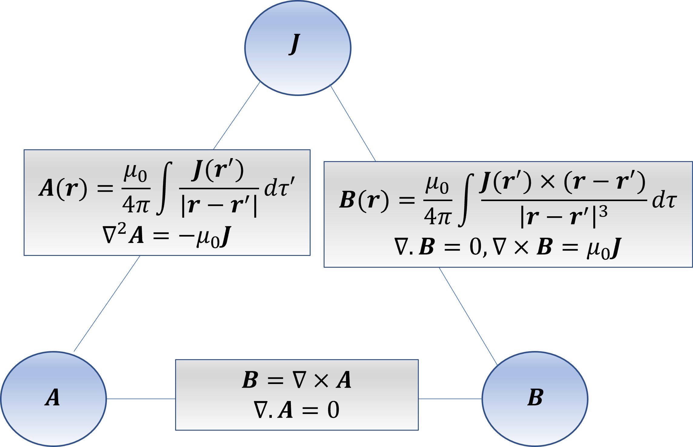
As before, if we know any of \(\vec{B}\), \(\vec{A}\) or \(\vec{J}\) we can determine the other. Note, however to find an \(\vec{A}\) from \(B\) is not easy (we have to incorporate the gauge (in this case \(\nabla\cdot \vec{A}\) ) into the calculation).