10. Electrodynamics - Faraday’s Law
So far, we have worked through the theory of electrostatics and magnetostatics and obtained equations, in terms of the divergence and curl of the fields, that relate the fields, \(\vec{E},\vec{B}\) to their sources \(\rho\) and \(\vec{J}\) and the associated fundamental constants \(\epsilon_0\) and \(\mu_0\).The origin of these equations is from careful experiments in the 19th century that established the source of the fields in terms of charge and current. By themselves there is nothing to suggest, so far, that they are related apart from their association with charged particles.
As the 19th century progressed and the experimental work continued, it was observed, especially in the work of Faraday, that changing magnetic fields actually give rise to an electromotive force that can be associated with the generation of an electric field. It is this observation, that changing magnetic fieilds give rise to electric fields, that we are going to explore now. We will explore later the relationship between time varying electric fields and magnetic fields as this is far more difficult to observe experimentally and is introduced as a theoretical concept in the first instance.
10.1 Potential difference and current.
When we discussed potential difference we explained that metals are equipotential surfaces as the free charges within them will always move in the presence of a field in such a way that the charge separation it produces creates a field that cancels the external field. We didn’t say anything about the currents that are produced as this redistribution of charges takes place. The flow of charge in our wires (or elsewhere) is called the current. Apart from the special case of superconductors, the charges (electrons) in metals do not flow freely but meet some resistance (we won’t go into the mechanisms here). Now, what happens if we maintain a steady (externally generated) potential difference across a wire? Well, the field generated by the potential will continually drive current through the wire (as it tries to equalise the field in the metal). Provided we can maintain the potential difference (if we had a battery say, it would eventually become exhausted and the metal ‘wins’ the contest in trying to zero the field across it), we maintain a steady current. The magnitude of this current is given by Ohm’s law,
\(\displaystyle V=I\,R\),
with which, I hope, you are familiar. Note, this law is not universal, there are some materials, e.g. semiconductors for which Ohm’s law in this simple form does not apply.
In terms of the current density (that we saw was important in describing magnetostatics fully, we can reformulate Ohm’s law to (see Griffiths 7.1.1.),
\(\displaystyle \vec{J}=\sigma\vec{E}\),
where, \(\sigma\) is known as the conductivity of the metal. From school, you may be more familiar with the concept of resistivity, that is just \(\rho = 1/\sigma\). Note, \(\sigma\) and \(\rho\) are the very common symbols usually used for conductivity and resistivity. They are not to be confused with surface charge density and volume charge density, that we used in electrostatics. We will not use resistivity and conductivity much but beware of any confusion! It is usually clear from the context what we are referring to but if you find this hard you might introduce your own symbols (say \(\rho_{\Omega}\) and \(\sigma_{\Omega}\)) to distinguish them.
Exercise. Show that you can recover Ohm’s law (\(V=IR\)) from the expression above, \(\vec{J}=\sigma\vec{E}\).
10.2 The Electromotive force (e.m.f.)
In the previous section we saw that the current is caused to flow by a force (often expressed as the force per unit charge \(\vec{f}\)) from an electric field \(\vec{E}\). Without any further input the currents would flow until the net field in the wire and \(\vec{f}\) become zero. So how do we describe the effects of a battery, that maintains a potential difference across the wire and continues to drive the current? This extra force \(\vec{f_s}\) must come from the battery so that, at any point we have
\(\displaystyle \vec{f}=\vec{f_S}+\vec{E}\),
where \(\vec{E}\) comes from any static fields in the circuit and \(\vec{f_s}\) comes from the source (for example, a battery, but other sources could include photocells, thermoelectric generators, piezo electricity etc.). Note, \(\vec{E}\) would continually adjust to zero if any imbalance started to build up. Whatever the origin of \(\vec{f_s}\) the net force around the circuit is,
\(\displaystyle \epsilon = \oint\vec{f} \cdot d\vec{l}=\oint\vec{f_s}\cdot d\vec{l}\),
as we note that for the static field \(\vec{E}\) we must have \(\oint\vec{E} \cdot d\vec{l}=0\). \(\epsilon\) is known as the electomotive force and is the net force per unit charge when integrating around the circuit. The origin of the force could be electrochemical (batteries), temperature difference (thermoelectrics) etc. and it is needed to sustain the current (unless the wire is superconducting).
For an ideal source ( i.e. a battery with no internal resistance) the net force on the charges when there is no connecting wire (\(\sigma_\Omega =0\)) is zero, so we expect \(\vec{E}=-\vec{f_s}\). Hence the potential difference \(V\) across the battery is,
\(\displaystyle V = -\int_a^b\vec{E}\cdot d\vec{l}=\int_a^b\vec{f_s}\cdot d\vec{l}=\oint\vec{f_s} \cdot d\vec{l}=\epsilon\),
where \(a\) and \(b\) represent the terminals of the battery. In electronics the e.m.f. would be known as the open circuit voltage. Note, also that \(\vec{f_s}\) is zero outside the battery.
10.3 Motional e.m.f.
In the previous section we considered the e.m.f. as coming from e.g. batteries. However, experiments, in particular those of Faraday, showed that e.m.fs could also be produced by changing magnetic fields. Consider the following figure,
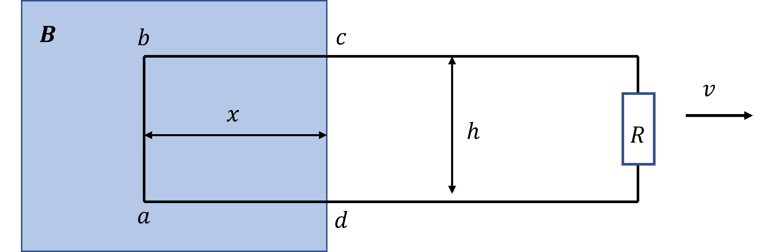
where the blue shaded region represents a region of uniform magnetic field pointing into the page. \(R\) is a resistor or ‘load’ on the circuit. In the absence of a static \(\vec{E}\) field, as the wired is pulled outwards (towards the right) a Lorentz force from the magnetic field is generated on the charge carriers in the wires. From the cross-priduct rule we see the charges in the segment \(ab\) of the wire feel a magnetic force \(qvB\) along the wire. (No steady current is created in the connecting segments). This force causes an e.m.f. to be generated in this section of the loop, such that,
\(\displaystyle \epsilon=\oint \vec{f}_{mag} \cdot d\vec{l}=v\,B\,h\)
where the integral represents a ‘snapshot’ in time. How does this e.m.f. generate work (i.e. heating the resistor) if magnetic fields do no work? The answer is the magnetic field is effective in transmitting the force but the work is done by whoever is pulling the wire. A good explanation about how this comes about is given, for example, in Griffiths example 5.3. For our purposes we just recognise that the changing field gives rise to an electromotive force. The size of the e.m.f. is often described in terms of the change in the magnetic flux as the wire passes through the field. The magnetic flux may be written (c.f. the electric flux) as,
\(\displaystyle \Phi =\int _A \vec{B}\cdot d\vec{a}\).
At any instant in time the flux in our loop of wire is \(\Phi_{loop}=Bhx\) so we find,
\(\displaystyle \frac{d\Phi}{dt}=Bh\frac{dx}{dt}=-Bhv\),
so finally we can equate the e.m.f. with the rate of change of the magnetic fluc within the circuit,
###You may be familiar with this from your school work. The minus sign is an expression of Lenz’s law, the change in flux opposes the induced e.m.f. An e.m.f. produced in this way is known as the motional e.m.f.
10.4 Faraday’s law.
Faraday carried out many experiments using different configurations of moving fields and wires and concluded that an e.m.f. was produced in any of the following circumstances,
when a wire loop is pulled out of a magnetic field (as described above),
if the loop was kept fixed and the magnetic field (say from a coil) was pulled away,
or, if the loop and position of the field were kept fixed but the magnetic field strength changed.
This leads to the conclusion that a changing magnetic field gives rise to an electric field (the e.m.f.).
If we combine the derivation of the e.m.f. in terms of the flux change in the circuit and the electric field \(\vec{E}\) in our circuit we find,
\(\displaystyle \epsilon =\oint\vec{E}\cdot d{l}=\frac{d\Phi}{dt}\),
or, in terms of the changing magnetic field,
\(\displaystyle \oint\vec{E}\cdot d\vec{l}=-\int_A\frac{\partial\vec{B}}{\partial t}\cdot d\vec{a}\).
This is known as Faraday’s law in integral form. If we apply Stoke’s theorem to the left hand-side of this equation we get,
###This is Faraday’s law in differential form and modifies our electrostatic result in the case of time varying magnetic fields. This is the third of Maxwell’s equations.
The key observation we have made here is that when we consider time varying fields there is a connection between what we thought of two distinct fields (\(\vec{E}\) and \(\vec{B}\)) previously, suggesting a connection between them.