12. Electrodynamics - the Displacement current.
12.1 Inconsistencies in our equations so far
In the last section we saw how magnetic fields that varied in time gave rise to electric fields and we saw how that modified our result for the curl of the electric field. So, so far we have,
\(\displaystyle \nabla \cdot\vec{E}=\frac{\rho}{\epsilon_0}\)
\(\displaystyle \nabla\cdot \vec{B}=0\)
\(\displaystyle \nabla\times\vec{E}=-\frac{\partial \vec{B}}{\partial t}\)
\(\displaystyle \nabla \times \vec{B}=\mu_0 \vec{J}\)
These equations are in essence the conclusion from the experiments of Ampere, Faraday etc. but are they complete? If something is missing why wasn’t an experimental effect observed.
Firstly for symmetry or aesthetic reasons you might wonder why there isn’t an effect from time dependent electric fields (\(\displaystyle \frac{\partial \vec{E}}{\partial t}\)) in a similar way to \(\displaystyle \frac{\partial \vec{B}}{\partial t}\). But is this all?
It was Maxwell who looked at these equations theoretically and observed an inconsistency. So we can try and follow his reassoning. So first, let’s ask, what is \(\nabla \cdot (\nabla \times \vec{E})\)? Well, from what we have,
\(\displaystyle \nabla \cdot (\nabla \times \vec{E})=\nabla \cdot \left(-\frac{\partial \vec{B}}{\partial t}\right)= -\frac{\partial }{\partial t} (\nabla \cdot\vec{B})\)
Well we know from our vector identities that the divergence of a curl is always zero. But as \(\nabla \cdot \vec{B}=0\) this doesn’t show any inconsistency. Bow what about \(\nabla \cdot(\nabla \times \vec{B})\)? Well, this should also be zero but we have,
\(\displaystyle \nabla \cdot (\nabla \times \vec{B})=\mu_0 (\nabla \cdot \vec{J})\)
Now, although we saw \(\nabla \cdot \vec{J} =0\) for the case of steady currents, it is not true for time dependent currents. So, as the left-hand side of our equation must be zero, it suggests there is something missing in our result for \(\nabla \times \vec{B}\). What might be missing?
Well, let’s look at the figure below,
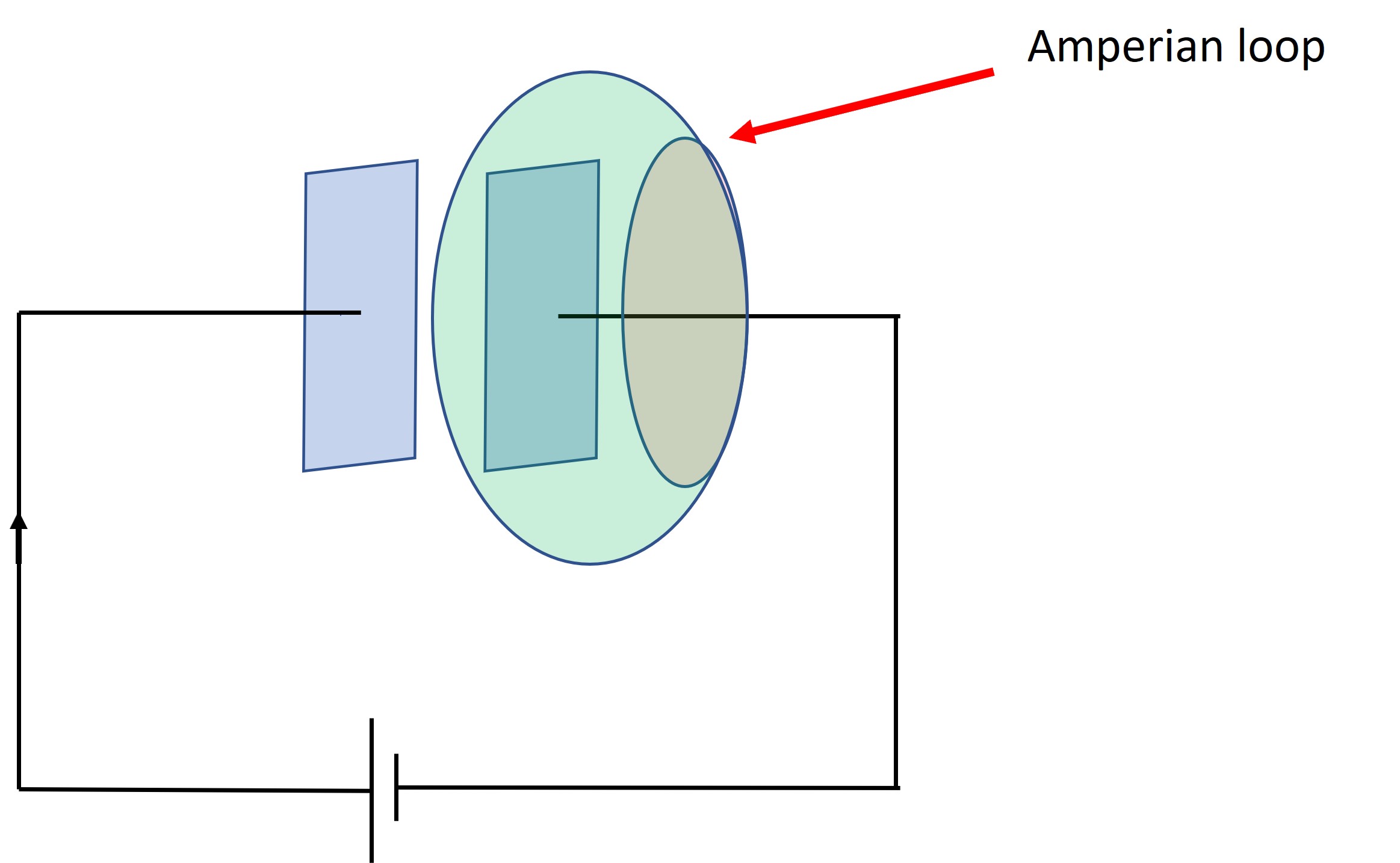
The figure shows a battery connected to a capacitor. In its final state the circuit would produce steady net charges on the plates of the capacitor - its an electrostatic system. Now, let’s ask what if we ask about how the capacitor becomes charged. To do this a current must flow in the wires to the capacitor. We can also work out (do it as an exercise) that the current, decays exponentially from its initial value until the capacitor becomes fully charged. That is the current in the wires is not steady. Nevertheless, this current will produce a magnetic field that we know, from Amperes law should have the property \(\displaystyle \oint \vec{B}\cdot d\vec{l} =\mu_0 I_{enclosed}\). Hopefully you will now see a difficulty. If my closed integral goes ‘around’ the current carrying wire, everything is fine. If I take my loop close to the capacitor plates (the small brown circle) it suggests there is a \(\vec{B}\) field present. However, if I shift by integration loop so that it is just inside the capacitor, Ampere’s law would suggest the field is zero! Do I really get a step change? Our arguments before also said the path I took in Ampere’s laws didn’t matter either. In other words something is not right!
To solve the problem we need to go back to our discussion of \(\nabla \cdot \vec{J}\) in terms of the continuity equation (see section 7.6). What happens when we have a time dependent charge distribution (i.e. the capacitor above charging)? Well,
\(\displaystyle \nabla \cdot \vec{J} = -\frac{\partial \rho}{\partial t}=-\frac{\partial}{\partial t}\left( \epsilon_0 \nabla \cdot \vec{E} \right)=-\nabla \cdot \left( \epsilon_0 \frac{\partial \vec{E}}{\partial t}\right)\)
where we’ve used \(\displaystyle \nabla \cdot \vec{E}=\frac{\rho}{\epsilon_0}\).
The right had term suggests that time varying electric fields also seem to behave like currents! So, to be complete, our expression for \(\nabla \times \vec{B}\) also needs to include this terem. From this, we arrive at the final result,
###.
This solves our inconsistency. Hoe does this apply to the figure above? Well, if we use an imaginary ‘curl meter’ we see that it will register a value if we are in the current carrying wire, but, if we are in the space between the capacitor plates it sees the time dependent \(\vec{E}\) filed that seems to behave as a current.
Because of its current like behaviour this extra term is known as the \(\textit Displacement current\) (or Maxwell’s displacement current), \(\vec{J}_d\) where,
\(\displaystyle \vec{J}_d=\epsilon_0 \frac{\partial \vec{E}}{\partial t}\).
With this result we can modify Ampere’s law as,
\(\displaystyle \oint \vec{B}\cdot d\vec{l}=\mu_0 I_{enclosed}+\mu_0\epsilon_0\int \left( \frac{\partial \vec{E}}{\partial t}\right) \cdot d\vec{a}\)
for the case of time dependent fields.
You might ask why, if we easily saw the effects of \(\partial \vec{B}/ \partial t\), in experiments, whe we didn’t see the effects of \(\partial \vec{E} / \partial t\)? Well, \(\mu_0 \epsilon_0\) is a very small number! However, with very careful experiments it is possible to observe this effect.
12.2 Maxwell’s equations
So we’ve now arrived at our destination and we can write the complete set of equations (Maxwell’s equations) for electromagnetism as,
###Some people like to write these by keeping the fields and their sources on either side of the equations, e.g.
###it’s up to you.
Along with the Lorentz force,
###\(\displaystyle \vec{F}=q(\vec{E}+\vec{v}\times\vec{B})\)
these define the equations of classical electromagnetism.
12.3 Where do you go from here with Maxwell’s equations ?
Maxwell’s equations lead to a remarkably rich set of phenomena. They let us understand how the electromagnetic force is transmitted over a distance, the time it takes and how the energy is transported. It is beyond this course to go any further. However, there is one more thing I’d like to show you that comes out reasonably straight forwardly and it is this.
Suppose we are in a region where there are no free charges (\(\rho=0\)) or currents (\(\vec{J}\). What happens if we look at the curl of \(\nabla \times \ \vec{E}\) and \(\nabla \times \vec{B}\)? (Remember how we looked at the divergence to get the Displacement current).
\(\displaystyle \nabla \times (\nabla \times \vec{E}) = \nabla (\nabla \cdot \vec{E})-\nabla ^2 \vec{E}\)
which is just the result of a vector identity you showed in the first problems class. Now if \(\rho = 0\) (so \(\nabla \cdot\ \vec{E}=0\)) in this region of space, this gives,
\(\displaystyle \nabla \times (\nabla \times \vec{E}) = \nabla (\nabla \cdot \vec{E})-\nabla ^2 \vec{E} = -\nabla^ 2\vec{E}\).
But we also have,
\(\displaystyle \nabla \times (\nabla \times \vec{E}) =\nabla \times -\frac{\partial \vec{B}}{\partial t}=-\frac{\partial}{\partial t}(\nabla \times \vec{B})\)
but, if \(\vec{J}=0\) (in this region of space), we can substitute for \(\nabla \times \vec{B}\) to get,
\(\displaystyle \nabla^2 \vec{E}=\mu_0\epsilon_0\frac{\partial ^2 \vec{E}}{\partial t^2}\)
Exercise, show how you can get a similar result for the \(\vec{B}\) field.
You should recognise this as the wave equation for the three components of \(\vec{E}\). That is Maxwell’s equations predict electromagnetic waves. I’ll leave you to work out their velocity and its significance.