11. Electrodynamics - induced electric fields
As we have progressed through our discussion of electromagnetism we have seen the importance of the the results that we found for the divergence and curl of the electric and magnetic field. Then, in the last section we begain to see, through our discussion of Faraday’s law the connection between the electric field and a time varying magnetic field. However, our expressions for the divergence and curl are still not quite complete. In the next few sections we will consider the symmetry we might expect in these equations - for example, we haven’t asked ourselves yet, what happens in the case of a time varying electric field. For the latter case there were no results from experimental measurements (we’ll see why later) that pointed to the solution.
11.1 Induced electric fields
Let’s consider the electromagnetic case where we are away from any free charges. In this case we would have,
\(\displaystyle \nabla\cdot \vec{E}=0\) ; \(\displaystyle \nabla \times \vec{E}=-\frac{\partial \vec{B}}{\partial t}\)
We can compare this with the result we obtained for the magnetic field,
\(\displaystyle \nabla \cdot \vec{B}=0\) ; \(\displaystyle \nabla \times \vec{B}=\mu_0 \vec{J}\)
Looking at this we can see that the changing magnetic field generates an \(\vec{E}\) field in exactly the same way as a current generates the \(\vec{B}\) field. Hence, we can think of an analog for the generation of the electric field in terms of what we found in the Biot-Savart law for \(\vec{B}\) by direct substitution of \(\vec{B}\) for \(\vec{E}\) and \(\mu_0\vec{J}\) for \(-\frac{\partial \vec{B}}{\partial t}\). This gives us the result,
\(\displaystyle \vec{E(\vec{r})}=-\frac{1}{4\pi}\int \frac{(\frac{\partial \vec{B(\vec{r'})}}{\partial t})\times (\vec{r}-\vec{r'})}{|\vec{r}-\vec{r'}|^3}d \tau'\)
or,
\(\displaystyle \vec{E(\vec{r})} =-\frac{1}{4\pi}\frac{\partial}{\partial t}\int \frac{\vec{B}\times (\vec{r}-\vec{r'})}{|\vec{r}-\vec{r'}|^3}d\tau'\).
By analogy, we also see that the role of the enclosed current in Ampere’s law for \(\vec{B}\), (\(\oint \vec{B}\cdot d\vec{l}=\mu_0 I_{enc}\)) is taken by the rate of change of the magnetic flux in Faraday’s law for the \(\vec{E}\) field as,
\(\displaystyle \oint\vec{E}.d\vec{l}=-\frac{d \Phi}{dt}\)
We should keep these analogies in mind as we progress.
11.2 Mutual Inductance.
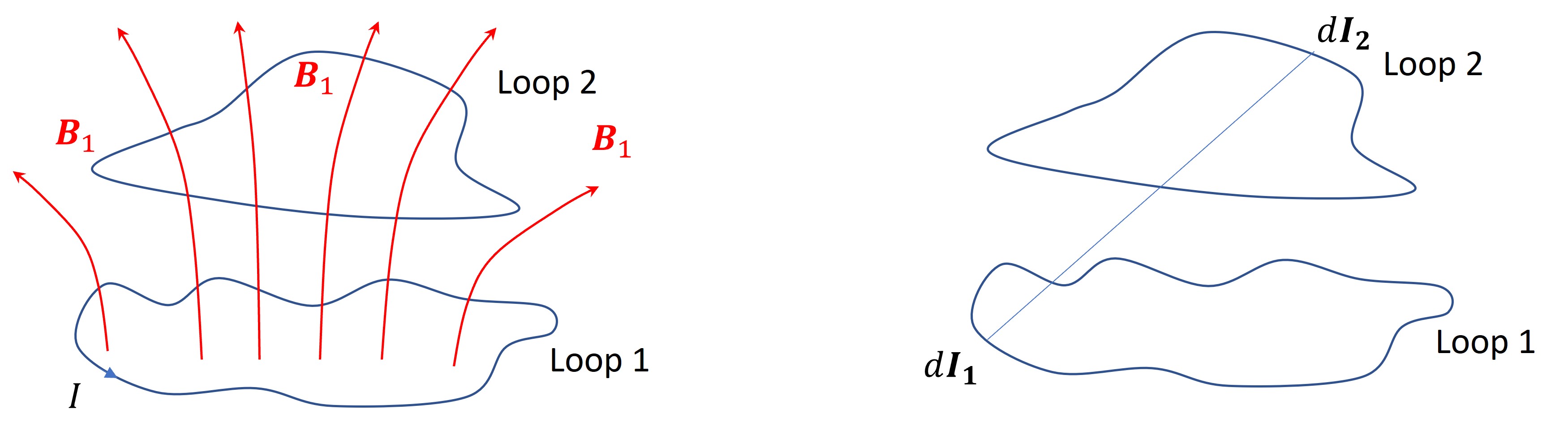
Consider the figure above. Suppose we have a current that is flowing in loop 1 and varying in time. This will generate a magnetic field in space, \(\vec{B_1}\), that is also varying in time. According to Faraday, this time varying field will induce an e.m.f. and hence a current in a nearby wire loop (loop 2). We express this in saying that the flux from coil 1 is linked to that in coil 2. This gives a simple description of the idea of mutual inductance (we could also consider a current in loop 2 generating an e.m.f. in loop 1).
Let’s look at this in a little more detail. In terms of the current in loop 1, we can write, using the Biot-Savart law,
\(\displaystyle \vec{B_1}=\frac{\mu_0}{4\pi}I_1 \oint \frac{d\vec{l_1}\times (\vec{r}-\vec{r'})}{|\vec{r}-\vec{r'}|^3}\)
From this expression it would be difficult, in all but the simplest cases, to calculate the flux of \(\vec{B_1}\) that passes through loop 2,
\(\displaystyle \Phi_2=\int \vec{B_1}\cdot d\vec{a}\).
However, we can see that \(\Phi_2\) will be proportional to \(I_1\), where the constant of proportionality depends on the geometrical arrangement of the coils. This constant of proportionality is known as the mutual inductance \(M_{21}\) so that,
\(\displaystyle \Phi_2 =M_{21}I_1\)
Can we obtain an expression for \(M_{21}\)? Well, with the help of our result for the magnetostatic potential (see section 8.6), we can write,
\(\displaystyle \Phi_2 = \int\vec{B_1}.d\vec{a_2}=\int(\nabla\times \vec{A_1})\cdot d\vec{a_2}=\oint \vec{A_1}\cdot d \vec{l_2}\),
where we have used Stoke’s theorem to get the line integral. But we also had (again section 8.6 and using the Coulomb gauge),
\(\displaystyle \vec{A_1}=\frac{\mu_0}{4\pi}I_1 \oint \frac{d\vec{l_1}}{|\vec{r}-\vec{r'}|}\).
From this we obtain,
\(\displaystyle \Phi_2 =I_1\;\frac{\mu_0}{4\pi}\oint \left(\oint \frac{d \vec{l_1}}{|\vec{r}-\vec{r'}|}\right).d\vec{l_2}\),
that gives us the result
###This is known as \(\textit{Neumann's formula}\). \(M_{21}\) is usually difficult to calculate from this expression but is ‘easy’ to measure. Two things that can be noted, - \(M_{21}\) only depends on the geometry and shapes of the loops, - \(M_{21}=M_{12}\) so the subscripts are normally dropped and the mutual inductance just known as \(M\).
From Faraday’s law we find the e.m.f. generated in the second loop from varying current in the first loop is,
###11.3 Self Inductance
If we consider a single wire loop carrying a current, we know, from Lenz’s law that any change in the current in the wire will cause an e.m.f. to oppose the change of current. In an analogous way to our treatment of mutual inductance we now define the link between the current in the loop and the flux through it itself as the self inductance, such that,
\(\displaystyle \Phi_1 =L\;I_1\)
from which we get the ‘back e.m.f.’ in the loop from the changing current as,
###The unit of inductance is the Henry where,
\(1 H = 1 V\cdot s\cdot A^{-1}\)
Aside. In the lectures we have now seen what are termed the ‘passive’ components in electronic circuits, namely, resistors (\(R\)), Capacitors (\(C\)) and Inductors (\(L\)). Their behaviour is very important, especially when we consider alternating currents so at the end of this series of lectures we will gather their properties together and show how we calculate circuit behaviour from these basic properties.
11.4 Energy in magnetic fields
If you have ever tried or seen someone try to cut the current suddenly in a large coil you soon realise there is a lot of energy released when the current is suddenly interrupted. See for example, induction coils and the care that needs to be taken to avoid damaging e.m.f.s when relays are switched. The power needed to increase the current is given by (c.f. \(P=I\;V\)),
\(\displaystyle P=\frac{dW}{dt}=-\epsilon\;I=LI\frac{dI}{dt}\)
If we start from zero current in the coil and build it up over time \(T\) the the energy stored in the coild may be found by intergarting this expression to give,
###.
This can be compared with the energy stored in a capacitor as \(W=\frac{1}{2}C\,V^2\).)
In the same way as we could imagine the energy stored in our capacitor as the energy asociated with the electric field, over all space, we can similarly show (see Griffiths section 7.2.4),
###